Interactive wxmplot displays

The wxmplot Overview describes the main features of wxmplot and shows how wxmplot plotting functions give a richer level of customization and interactivity to the end user than is available from the standard matplotlib.pyplot when run from a script or program.

Here, the emphasis is on the immediacy of the interactivity of the data displays especially when used from interactive sessions, including plain Python REPL, IPython/Jupyter console, Jupyter Notebooks, or the Python Kernel in Jupyter Lab.

An important feature of the plot(), imshow() and other functions of the interactive module in general is that they display their results immediately, without having to execute a show() method to render the display. For interactive work from the Python REPL or one of the Jupyter prompts, the displayed windows do not block the Python session. This means that not only can you zoom in, change themes, etc from the Plot window, you can can also easily plot other functions or data, either on the same window or in a new top-level plotting window.

For Jupyter Notebooks, it should be noted that while other plotting libraries (matplotlib, plotly, and bokeh) will show graphics in-line, as part of the Notebook, wxmplot will use separate display windows, outside of the browser. Having the visual display of data outside the notebook can be considered an advantage, While the interactive plots are then not saved directly within the Notebook, the code to generate the plots can be re-run. And images of the plot results can be copied and pasted as Markdown cells.

The functions in the interactive are described in detail below. While the functions plot(), imshow() are roughly equivalent to those in matplotlib.pyplot, they are not exact drop-in replacements for the pyplot functions.

Plotting in an interactive session or Jupyter

As an example using wxmplot.interactive in a Jupyter console session might look like this:

~> jupyter console
Jupyter console 6.6.3

Python 3.13.9 | packaged by conda-forge | (main, Oct 22 2025, 23:31:04) [Clang 19.1.7 ]
Type 'copyright', 'credits' or 'license' for more information
IPython 9.7.0 -- An enhanced Interactive Python. Type '?' for help.
Tip: Use `%timeit` or `%%timeit`, and the  `-r`, `-n`, and `-o`
option    s to easily profile your code.

In [1]: import numpy as np
In [2]: import wxmplot.interactive as wi
In [3]: x = np.linspace(0, 20, 101)
In [4]: wi.plot(x, np.sin(x), xlabel='t (sec)')
Out[4]: <wxmplot.interactive.PlotDisplay at 0x11ef74290>

At this point a plot like this will be displayed:

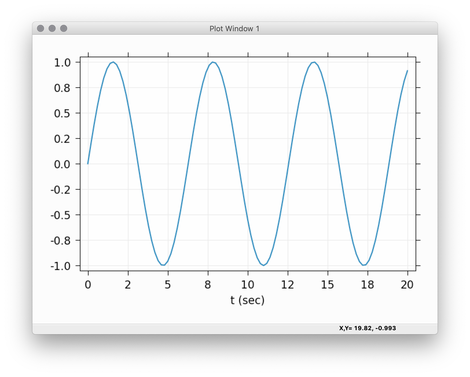
The wxmplot display will have full interatvity and can be configured after it is drown.

For example, from the Plot Configuration window we could change the theme to ‘Seaborn’ and set the label for this trace to be ‘sine’. Then from the Jupyter console we can continue:

In [5]: wi.plot(x, np.cos(1.5*x), label='cosine', show_legend=True)
Out[5]: <wxmplot.interactive.PlotDisplay at 0x10db88678>

which will now show:

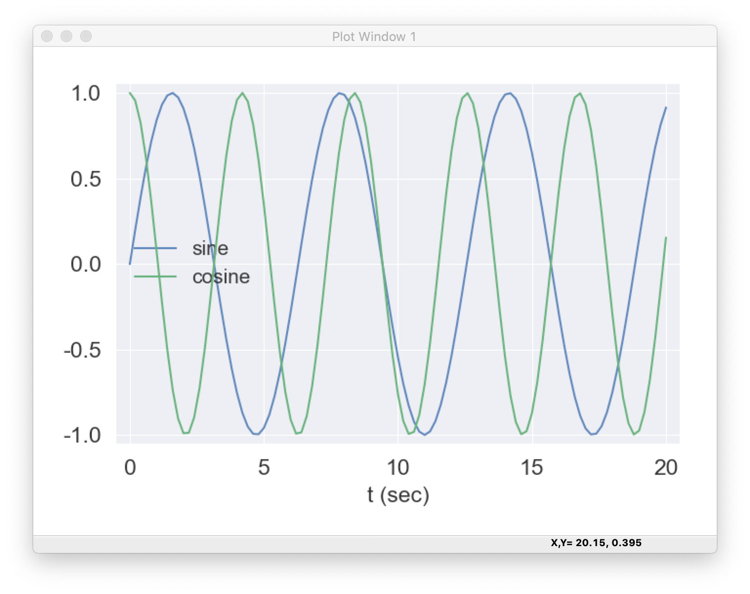
which is again a fully interactive and configurable display. For example, with the legend displayed, clicking on any of the labels in the legend will toggle the display of that curve. If we want to clear the data and plot something new, we might do something like:

In [6]: wi.plot(x, x*np.log(x+1), label='xlogx', new=True)
Out[6]: <wxmplot.interactive.PlotDisplay at 0x10db88678>

We can also place a text string, arrow, horizontal, or vertical line on the plot, as with:

In [7]: wi.plot_text('hello!', 9.1, 0.87)

and so forth.

If we wanted to bring up a second Line Plot window, we can use the win=2 option:

In [8]: wi.plot(x, np.sin(x)*np.exp(-x/8) , win=2, theme='ggplot')
Out[8]: <wxmplot.interactive.PlotDisplay at 0x110b2fb88>

and then control which of the displays any additional plot functions use by passing the win option to the plotting functions.

The immediacy of the rendering and the ability to customize the plots makes these plotting functions well-suited for exploratory displays of data.

Examples of ipython notebook files are included in the examples folder.

Using the interactive functions from a script

When using the interactive functions in a script or program that is run in a non-interactive way, say from a commandline shell, the wxmplot displays will still appear. The act of plotting will not block further execution of the script, and the script will continue to run, possibly making more wxmplot displays. When the script reaches is end, the displays will not be automatically closed. Instead, the plots and images will remain displayed and fully interactive until all windows have been closed or until the running script is explicitly closed (say, with Ctrl-D). That means that you can add wi.plot() and wi.imshow() to your scripts and the plots will be displayed until you no longer want to use them.

Line Plotting with plot() and related functions

wxmplot.interactive.plot(x, y, win=1, new=False, ...)

Plot trace of x, y arrays in a PlotFrame

Parameters:

• x (array-like) – ordinate values [0]

• y (array-like, None) – abscissa values (x and y must be same size!) [0]

• dy (array-like) – array for error bars in y (must be same size as y!)

• new (bool) – whether to start a new plot [False]

• win (int) – index of Plot Window [1]

• label (str or None) – label for this trace

• linewidth (float) – width of line joining points [from theme]

• color (str or None) – color for trace (see note 1) [from theme]

• style (str or None) – line style for joining points (see note 2)

• marker (str on None) – symbol to draw at each point (see note 3)

• markersize (float) – size of marker

• zorder (float or None) – zorder (depth) of this trace

• drawstyle (str or None) – style for joining line segments (see note 4)

• xmin (float or None) – minimum x value for plot range

• xmax (float or None) – maximum x value for plot range

• ymin (float or None) – minimum y value for plot range

• ymax (float or None) – maximum y value for plot range

• use_dates (bool) – whether to interpret x data as dates [False]

• side (str) – side for y-axis (‘left’ or ‘right’) [‘left’]

• size (tuple or None) – width, height in pixels of Plot Window

• wintitle (str or None) – title for window frame

• theme (str on None) – plotting theme to use

• title (str or None) – plot title

• xlabel (str or None) – label for x-axis

• ylabel (str or None) – label for y-axis

• y2label (str or None) – label for y2-axis (that is, right-side axis)

• xlog_scale (bool) – whether to show x-axis as log-scale [False]

• ylog_scale (bool) – whether to show y-axis as log-scale [False]

• grid (bool) – whether to draw background grid [True]

• show_legend (bool or None) – whether to show legend [False]

• legend_loc (str) – location for legend (see note 5) [‘best’]

• legend_on (bool) – whether legend is within the main axes [True]

• bgcolor (str on None) – color of background plot area (from theme)

• framecolor (str on None) – color of outer frame area (from theme)

• gridcolor (str or None) – color of grid (from theme)

• labelfontsize (float) – size (pixels) of font for Labels (from theme)

• legendfontsize (float) – size (pixels) of font for Legend (from theme)

• titlefontsize (float) – size (pixels) of font for Title (from theme)

• axes_style (str) – control what parts of axes are shown (see note 6)

• viewpad (float or None) – percent of data range to expand view ranges

• delay_draw (boole) – whether to delay drawing [False]

Returns:

plotter, a PlotFrame

Notes

0. If y is None (or not provided), the array for x becomes y, and x will be set to the array index: np.arange(len(y))

1. colors can be names such as ‘red’ or hex strings ‘#RRGGBB’. by default, they are set by the theme

2. styles can be one of ‘solid’, ‘short dashed’, ‘dash-dot’, ‘dashed’, ‘dotted’, ‘long-dashed’.

3. markers can be one of ‘no symbol’, ‘o’, ‘+’, ‘x’, ‘square’, ‘diamond’, ‘thin diamond’, ‘^’, ‘v’, ‘>’, ‘<’, ‘|’, ‘_’, ‘hexagon’, ‘pentagon’, ‘tripod 1’, or ‘tripod 2’

4. drawstyle can be one of ‘default’, ‘steps-pre’,’steps-mid’, or ‘steps-post’.

5. legend_loc can be one of ‘best’, ‘upper right’ , ‘lower right’, ‘center right’, ‘upper left’, ‘lower left’, ‘center left’, ‘upper center’, ‘lower center’, ‘center’

6. axis_style can be one of ‘open’, ‘box’, ‘bottom’.

More details of Plot Options are given in Table of Plot Arguments.

wxmplot.interactive.hist(x, bins=10, win=1, new=False, size=None, force_draw=True, title=None, *args, **kws)

display a histogram

Parameters:

• x (array-like) – array of values

• bins (int) – number of bins to show

• win (int) – index of plot window

wxmplot.interactive.update_trace(x, y, trace=1, win=1, **kws)

update a plot trace with new data, avoiding complete redraw This can significantly descrease drawing time:

Parameters:

• x (array-like) – ordinate values

• y (array-like) – abscissa values (x and y must be same size)

• trace (int) – which plot trace to update [1]

• win (int) – index of Plot Window [1]

• side (str) – side for y-axis (‘left’ or ‘right’) [‘left’]

wxmplot.interactive.set_data_generator(data_generator, polltime=25, win=1)

Set data generator function or generator for a plot window that will be called to generate new data to be displayed. The generator or data-generating funcion will be call at intervals set by polltime

Parameters:

• data_generator: – callable function that will return or yield data to plot.:

• polltime (time in ms to wait for polling [default=25])

Return type:

plot window

Notes

the generator function takes no arguments (but can be a partial) and must return either None to stop updating, or a list of pairs of x, y that update each trace in the plot.

To update a single dataset, your function should return with

return [(xnew, ynew)]

or generator yield with

yield [(xnew, ynew)]

to update mulitple traces, your function or generator should

return [(xnew, ynew), (xnew, y2new)]

or

yield [(xnew, ynew), (xnew, y2new)]

wxmplot.interactive.plot_setlimits(xmin=None, xmax=None, ymin=None, ymax=None, win=1)

set plot view limits for plot in window win

Parameters:

• xmin (float) – minimum x value

• ymax (float) – maximum x value

• ymin (float) – minimum y value

• ymax – maximum y value

• win (int) – index of plot window

wxmplot.interactive.plot_text(x, y, text, win=1, options)

add text at x, y coordinates of a plot

Parameters:

• text (str) – text to draw

• x (float) – x position of text

• y (float) – y position of text

• win (int) – index of plot window

• rotation (str or float) – text rotation. angle in degrees or ‘vertical’ or ‘horizontal’

• ha (str) – horizontal alignment (‘left’, ‘center’, ‘right’)

• va (str) vertical alignment ('top', 'center', 'bottom', 'baseline')

• side (str) – which axis to use (‘left’ or ‘right’) for coordinates.

wxmplot.interactive.plot_arrow(x1, y1, x2, y2, win=1, **kws)

draw arrow from x1, y1 to x2, y2.

Parameters:

• x1 (float) – starting x coordinate

• y1 (float) – starting y coordinate

• x2 (float) – ending x coordinate

• y2 (float) – ending y coordinate

• side (str) – which axis to use (‘left’ or ‘right’) for coordinates.

• shape (str) – arrow head shape (‘full’, ‘left’, ‘right’)

• color (str) – arrow color (‘black’)

• width (float) – width of arrow line (in points. default=0.0)

• head_width (float) – width of arrow head (in points. default=0.05)

• head_length (float) – length of arrow head (in points. default=0.25)

• overhang (float) – amount the arrow is swept back (in points. default=0)

• win (int) – index of plot window

wxmplot.interactive.plot_marker(x, y, marker='o', size=4, color='black')

draw a marker at x, y

Parameters:

• x (float) – x coordinate for marker

• float) (y) – y coordinate

• marker (str) – symbol to draw at each point (see Note 1)

• size (float) – marker size [4]

• color (str) – marker color [‘black’]

• win (int) – index of plot window

Notes

1. marker can be one of (‘+’, ‘o’, ‘x’, ‘square’, ‘diamond’, ‘thin diamond’, ‘^’, ‘v’, ‘>’, ‘<’, ‘|’, ‘_’, ‘hexagon’, ‘pentagon’, ‘tripod 1’, or ‘tripod 2’)

wxmplot.interactive.plot_axhline(y, xmin=None, ymin=None, **kws)

plot a horizontal line spanning the plot axes

Parameters:

• y (float) – y position of line

• xmin (float) – starting x fraction (window units – not user units!)

• xmax (float) – ending x fraction (window units – not user units!)

• win (int) – index of plot window

wxmplot.interactive.plot_axvline(y, xmin=None, ymin=None, **kws)

plot a vertical line spanning the plot axes

Parameters:

• x (float) – x position of line

• ymin (float) – starting y fraction (window units – not user units!)

• ymax (float) – ending y fraction (window units – not user units!)

• win (int) – index of plot window

Displaying images with imshow() and contour()

wxmplot.interactive.imshow(map, ...)

Display an 2-D array of intensities as a false-color map

Parameters:

• map (ndarray) – map array data (see Note 1)

• y (array-like) – values for pixels along vertical direction

• x (array-like) – values for pixels along horizontal direction

• colormap (str) – name of colormap to apply

• win (int) – index of Image Window (1 to %d)

• size (tuple) – width, height in pixels of Image Window

• wintitle (str) – text for Window title [Image Window N]

• xlabel (str) – label for horizontal axis [‘X’]

• ylabel (str) – label for horizontal axis [‘Y’]

• style (str) – display style (‘image’ or ‘contour’) [‘image’]

• nlevels (int) – number of levels for contour

• contour_labels (bool) – whether to show contour labels [True]

• show_axis (bool) – whether to shos Axis [False]

• contrast_level (float or None) – percent level for contrast [‘0.1’]

Returns:

img, an ImageFrame

Notes

1. the map data can either be a 2d array (shape NY, NX) for single-color map or (NY, NX, 3) array for an RGB map

wxmplot.interactive.contour(map, ...)

Display an 2-D array of intensities as a contour plot

Notes

This is equivalent to imshow(map, …, style=’contour’)

Functions for working with the interactive windows

wxmplot.interactive.set_theme(theme)

set plotting theme by name with a theme name

Parameters:

theme (str) – name of theme

Returns:

None

Notes

1. Example themese are:’light’, ‘dark’, ‘white-background’, ‘matplotlib’, ‘seaborn’, ‘ggplot’, ‘bmh’, ‘fivethirtyeight’. 2. See available_themes() for the list of available themes.

wxmplot.interactive.available_themes()

list of available theme

Returns:

list of theme names.

Notes

As of this writing, the list is:

‘light’, ‘dark’, ‘white-background’, ‘matplotlib’, ‘seaborn’, ‘ggplot’, ‘bmh’, ‘fivethirtyeight’, ‘grayscale’, ‘dark_background’, ‘tableau-colorblind10’, ‘seaborn-bright’, ‘seaborn-colorblind’, ‘seaborn-dark’, ‘seaborn-darkgrid’, ‘seaborn-dark-palette’, ‘seaborn-deep’, ‘seaborn-notebook’, ‘seaborn-muted’, ‘seaborn-pastel’, ‘seaborn-paper’, ‘seaborn-poster’, ‘seaborn-talk’, ‘seaborn-ticks’, ‘seaborn-white’, ‘seaborn-whitegrid’, ‘Solarize_Light2’

wxmplot.interactive.get_wxapp(redirect=False, clearSigInt=True)

get the wx App

Parameters:

• redirect (bool) – whether to redirect output that would otherwise be written to the Console [False]

• clearSigInt (bool) – whether to clear interrupts of Ctrl-C [True]

Returns:

a wx.App instance

wxmplot.interactive.get_plot_window(win=1, size=None, wintitle=None, theme=None)

return a plot display

Parameters:

• win (int) – index of Plot Window (1 to 100)

• size (tuple) – width, height in pixels of Plot Window

• wintitle (str) – text for Window title [Plot Window N]

• theme (str) – theme for Plot Window [‘light’ or ‘dark’]

Returns:

diplay, a wxmplot PlotFrame.

Notes

this will either return the existing PlotFrame for the window index or create a new one.

The returned wx.PlotFrame from get_plot_window() will have the many attributes and methods, with some of the most useful described in the table below, Table of interactive Plot Window attributes and methods. This includes access to the underlying matplotlib Axes and Canvas objects.

wxmplot.interactive.get_image_window(win=1, size=None, wintitle=None)

return an image display

Parameters:

• win (int) – index of Image Window (1 to 100)

• size (tuple) – width, height in pixels of Image Window

• wintitle (str) – text for Window title [Image Window N]

Returns:

diplay, a wxmplot ImageFrame.

Notes

this will either return the existing ImageFrame for the window index or create a new one.

As with wx.PlotFrame, the returned wx.ImageFrame will have the same principle attributes to access the matplotlib Axes and Canvas objects.

Plot frame attributes and methods

Table of interactive Plot Window attributes and methods

name	object type
.cursor_history	[(x, y, timestamp), …] of cursor selections
.save_figure()	method to save image to a png file
.configure()	method to show Configuration window
.get_config()	method to return configuration dictionary
.set_config()	method to update configuration with keyword/values
.panel	wxmplot.PlotPanel, a wx.Panel
.panel.conf	wxmplot.PlotConfig
.panel.axes	matplotlib.axes.AxesSubPlot
.panel.fig	matplotlib.figure.Figure
.panel.canvas	matplotlib.backends.backend_wxagg.FigureCanvasWxAgg

Note that the cursor_history attribute will be a list of (x, y, timestamp) values with x and y being in “user coordinates, timestamp being the Unix timestamp for each even of pressing the left mouse button on the plot. The most recent event will be in cursor_history[0], and the list will be in descending time order. Only the most recent 100 cursor events will be retained.

Each new plot will clear the cursor_history.